Weibull models

Weibull models are a commonly used parametric survival or failure time model. These are notes to help the me understand Weibull models and remember what I learned. The main way I started to get a feel for Weibull models was to initally ignore issues arounding censoring.

In R, the Weibull distribution is parametized according to a shape parameter \(a\) and scale parameter \(b\) for \(x>0\) as follows:

\[ f(x) = (a/b) (x/b)^{(a-1)} \exp(- (x/b)^a) \]

This parameterization matches that of the "standard parameterization" on Wikipedia's Weibull page except Wikipedia uses \(k\) for the shape parameter \(\lambda\) for the scale parameter.

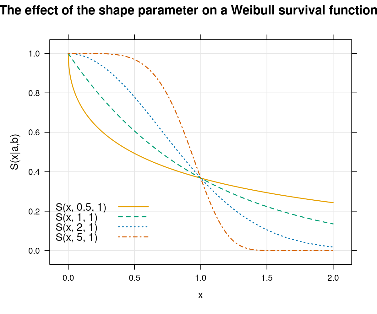
Shape parameter

The shape parameter can be seen to influence the survival function \(S(x|a,b) = 1 - F(x|a,b)\) in terms of whether it quickly or slowly decreases. With \(a<1\), \(S(x|a,b)\) drops quickly initially but then the rate of change of decreases. With \(a>1\), \(S(x|a,b)\) decreases slowly initially but then drops more quickly before eventually changing more slowing. Failure times associated with frequent early failure will have \(a<1\) while failure times associated with aging or another kind of wear-out process will have \(a>1\). Below are survival curves for multiple values of \(a\) fixing \(b=1\). (This plot shows a property that I do not remember reading about which is that for a given \(b\), all the survival curves intersect at \(x=b\).)

library(lattice)
mytheme <- simpleTheme(lwd = 1.5, 
                       lty = 1:4,
                       col = palette.colors(7)[c(2, 4, 6, 7)])

S <- function(x, shape, scale) {
    pweibull(x, shape, scale, lower.tail = FALSE)
}

x <- seq(0, 2, length = 500)

xyplot(S(x, 0.5, 1) + S(x, 1, 1) + S(x, 2, 1) + S(x, 5, 1) ~ x,
       ylab = "S(x|a,b)",
       main = "The effect of the shape parameter on a Weibull survival function",
       type = "l",
       par.settings = mytheme,
       auto.key = list(lines = TRUE, points = FALSE,
                       x = 0, y = 0.10, corner = c(0, 0)),
       as.table = TRUE,
       grid = TRUE)

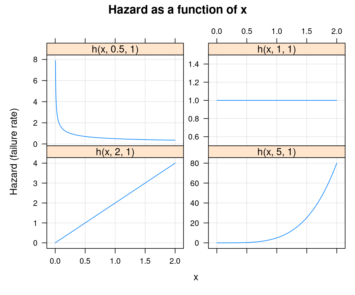
The hazard function represents the instantaneous failure rate and is defined as

\[ h(x|a,b) = f(x|a,b)/S(x|a,b) \]

In addition to the shape parameter influencing how \(S(x|a,b)\) is changing with x, its effect is more clearly seen in the hazard function. For \(a<0\) the hazard is decreasing (i.e., the failure rate is decreasing), for \(a=1\) it is constant, and for \(a>1\) it is increasing. A special case is when \(a=2\) for which the hazard is increasingly linearlly. Below are four panels showing the hazard function \(h(x|a,b)\) corresponding to the four survival curves above. (Since the hazards are on very different scales they are plotted in separate panels.)

library(lattice)
h <- function(x, shape, scale) {
    dweibull(x, shape, scale) /
    pweibull(x, shape, scale, lower.tail = FALSE)
}
xyplot(h(x, 0.5, 1) + h(x, 1, 1) + h(x, 2, 1) + h(x, 5, 1) ~ x,
       ylab = "Hazard (failure rate)",
       main = "Hazard as a function of x",
       type = "l",
       scales = list(y = list(relation = "free", rot = 0)),
       outer = TRUE,
       as.table = TRUE,
       grid = TRUE)
## x <- rweibull(100, shape = 2, scale = 5)
## histogram(~ x, main = "Weibull histogram", type = "density", ylim = c(0, 0.25))